Plotting

Below we describe additional features available for customising spectral plots.

Creating publication-quality plots

By default, the legend will be positioned to the right of the figure box with the best-fit parameter values and the full model name. The automated plotting includes an alternative, more compact figure style with the legend included within the figure box and with an abbreviated model name and no fit info. This is done by enabling alternate_style=True in find_best_spectral_fit():

from pulsar_spectra.catalogue import collect_catalogue_fluxes
from pulsar_spectra.spectral_fit import find_best_spectral_fit

cat_dict = collect_catalogue_fluxes()
pulsar = 'J1909-3744'
freqs, bands, fluxs, flux_errs, refs = cat_dict[pulsar]
best_model_name, iminuit_result, fit_info, p_best, p_category = find_best_spectral_fit(pulsar, freqs, bands, fluxs, flux_errs, refs, plot_best=True, alternate_style=True)

This will produce the following plot:

Using custom marker types

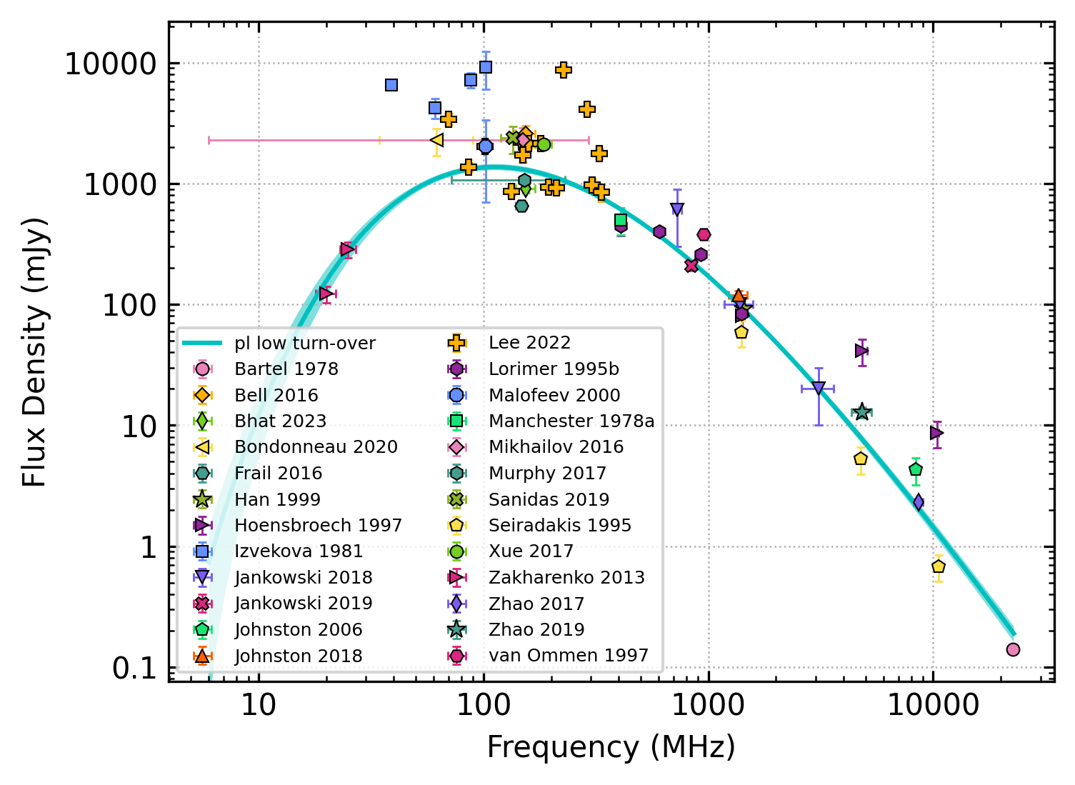
By default, the code will cycle through a set list of marker types. When creating figures for multiple pulsars, the default marker assignment can lead to inconsistency in the marker types. This can be solved by assigning a custom marker to each reference. You can specify custom marker types using the following code:

from pulsar_spectra.catalogue import collect_catalogue_fluxes
from pulsar_spectra.spectral_fit import find_best_spectral_fit

custom_markers = {
#   reference           :   (marker colour, marker type, marker size)
    "Jankowski_2018"    :   ('magenta', 'h', 5), # orange circle
    "Jankowski_2019"    :   ('cyan', 'H', 5)  # green diamond
}

cat_dict = collect_catalogue_fluxes()
pulsar = 'J1909-3744'
freqs, bands, fluxs, flux_errs, refs = cat_dict[pulsar]
best_model_name, iminuit_result, fit_info, p_best, p_category = find_best_spectral_fit(pulsar, freqs, bands, fluxs, flux_errs, refs, plot_best=True, ref_markers=custom_markers)

This will produce the following plot:

To generate a set of unique markers for any set of pulsars, see Generating a consistent marker set for a multi-pulsar plot.

Plotting a secondary model

Sometimes you may want to plot more than one best-fit model on the same figure with different subsets of data included in the fit. To differentiate between the two models, we have included an alternate model style which is light grey and does not show the uncertainty envelope. For example, the following code can be used to show the model fit before and after the addition of your data:

import matplotlib.pyplot as plt
from pulsar_spectra.catalogue import collect_catalogue_fluxes
from pulsar_spectra.spectral_fit import find_best_spectral_fit

cat_dict = collect_catalogue_fluxes()
pulsar = 'J1909-3744'
freqs, bands, fluxs, flux_errs, refs = cat_dict[pulsar]

fig, ax = plt.subplots(figsize=(5,4))
find_best_spectral_fit(pulsar, freqs, bands, fluxs, flux_errs, refs, plot_best=True, secondary_fit=True, axis=ax)

freqs = [150.] + freqs
bands = [30.] + bands
fluxs = [6.] + fluxs
flux_errs = [1.] + flux_errs
refs = ['Your Work'] + refs
best_model_name, iminuit_result, fit_info, p_best, p_category = find_best_spectral_fit(pulsar, freqs, bands, fluxs, flux_errs, refs, plot_best=True, axis=ax)

plt.savefig(pulsar+'_'+best_model_name+'_fit.png', bbox_inches='tight', dpi=300)

This will produce the following plot:

Creating a custom plotting configuration

The figure, marker, and model styles are specified in the pulsar_spectra/configs/plotting_config.yaml file. Customisation of the plotting configuration is made easy with the build_plotting_config.py script. Information about all available customisations can be found in the help menu:

build_plotting_config.py -h

The default configuration is created by omitting all command line inputs, which will write to a file called plotting_config.yaml in the current directory. If you customise the configuration and want to make it the new default, you can replace the default pulsar_spectra/configs/plotting_config.yaml and then reinstall pulsar_spectra from the base directory:

pip install .

If you would like to use a non-default configuration in your script, you can include it by giving the file path to plotting_config in find_best_spectral_fit() like so:

from pulsar_spectra.catalogue import collect_catalogue_fluxes
from pulsar_spectra.spectral_fit import find_best_spectral_fit

cat_dict = collect_catalogue_fluxes()
pulsar = 'J0953+0755'
freqs, bands, fluxs, flux_errs, refs = cat_dict[pulsar]
best_model_name, iminuit_result, fit_info, p_best, p_category = find_best_spectral_fit(pulsar, freqs, bands, fluxs, flux_errs, refs, plot_best=True, plotting_config='custom_plotting_config.yaml')

In the following example, we want to make the following customisations:

• Increase the figure width to 4 inches (keeping the default aspect ratio) (--fig_height 4)

• Change the line style of the primary model to a solid line (--primary_ls -)

• Change the colour of the model and model error regions to cyan (--model_colour c --model_error_colour c)

• Generate a set of unique and randomised markers with the IBM colour palette (--generate_markers --shuffle --palette IBM)

• Save the file as custom_plotting_config.yaml (-F custom_plotting_config.yaml)

This can be done with the command:

build_plotting_config.py \
--fig_height 4 \
--primary_ls - \
--model_colour c \
--model_error_colour c \
--generate_markers \
--shuffle \
--palette IBM \
-F custom_plotting_config.yaml

The result is the following plot

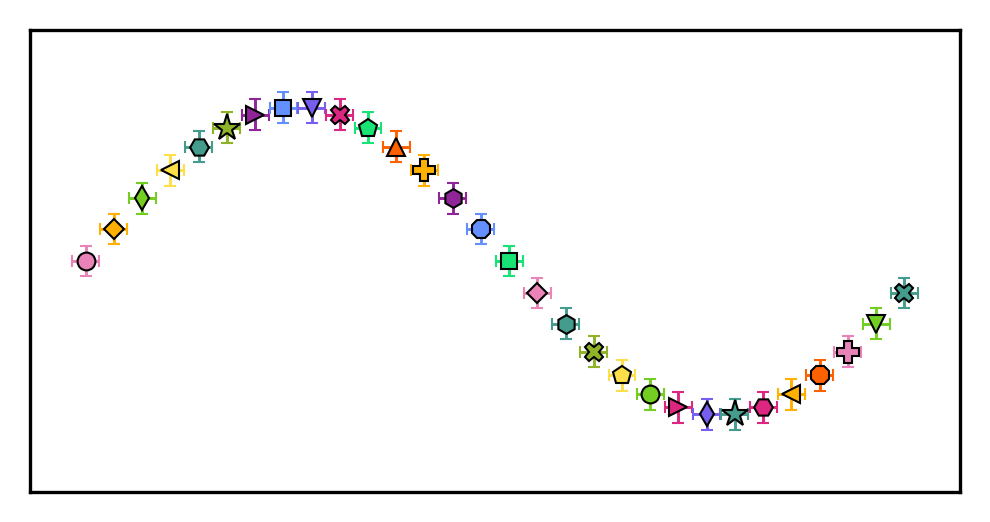
By default, the --generate_markers (or -g) option will create a set of 30 unique markers, which will be ordered based on the order of the colour palette and marker type lists (currently hard-coded in build_plotting_config.py). You can use the --num_markers option to increase the size of the unique marker set, and the --shuffle option to shuffle the order of markers and colours.

Note: the shuffle option is not completely random. All of the marker types will be used before a marker type is reused, and the same is true for the marker colours.

If you would like to save the generated marker set, you can use the --marker_file_savename option to specify a file to write to. This can then be imported with the --marker_file option. You can preview the generated marker set using --marker_preview, producing marker_preview.png:

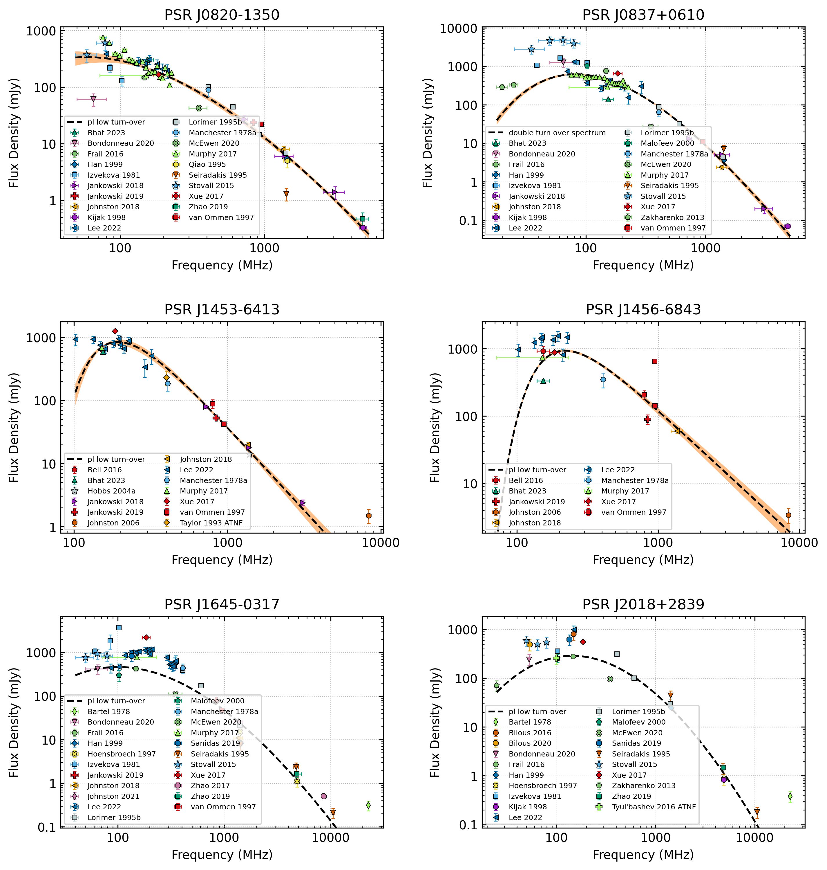
Generating a consistent marker set for a multi-pulsar plot

As discussed above, you may want to use a consistent set of markers when showing spectral plots side by side. This is made easy with the build_plotting_config.py script. To generate a consistent marker set for a set of pulsars, use the --pulsars (or -p) option. For example:

build_plotting_config.py \
--primary_ls - \
--model_colour c \
--model_error_colour c \
--generate_markers \
--shuffle \
--palette WONG \
-F custom_plotting_config.yaml \
-p J0820-1350 J0837+0610 J1453-6413 J1456-6843 J1645-0317 J2018+2839

In addition to custom_plotting_config.yaml, this will also generate ref_markers.yaml, You can then import them in a multi-pulsar plot like so:

import yaml
import matplotlib.pyplot as plt
from pulsar_spectra.spectral_fit import find_best_spectral_fit
from pulsar_spectra.catalogue import collect_catalogue_fluxes

with open('ref_markers.yaml', 'r') as f:
    ref_markers = yaml.safe_load(f)

pulsars = [
    'J0820-1350',
    'J0837+0610',
    'J1453-6413',
    'J1456-6843',
    'J1645-0317',
    'J2018+2839'
]

cols = 2
rows = 3
fig, axs = plt.subplots(nrows=rows, ncols=cols, figsize=(5*cols, 3.5*rows))

cat_dict = collect_catalogue_fluxes()
for ax_i, pulsar in enumerate(pulsars):
    freqs, bands, fluxs, flux_errs, refs = cat_dict[pulsar]
    model, m, fit_info, p_best, p_category = find_best_spectral_fit(pulsar, freqs, bands, fluxs, flux_errs, refs, plot_best=True, alternate_style=True, axis=axs[ax_i//cols, ax_i%cols], ref_markers=ref_markers)
    axs[ax_i//cols, ax_i%cols].set_title('PSR '+pulsar)

plt.tight_layout(pad=2.5)
plt.savefig("multi_pulsar_spectra.png", bbox_inches='tight', dpi=300)

This will produce multi_pulsar_spectra.png with consistent marker types:

If you add your own data as shown here, then you can add a custom marker for your own data by adding a new entry to the ref_markers dictionary. For example:

ref_markers["Your Work"] = ['green', 'o', 7]