Examples
Simple example
The following can be run to fit J0332+5434
from pulsar_spectra.catalogue import collect_catalogue_fluxes
from pulsar_spectra.spectral_fit import find_best_spectral_fit

cat_dict = collect_catalogue_fluxes()
pulsar = 'J0332+5434'
freqs, bands, fluxs, flux_errs, refs = cat_dict[pulsar]
best_model_name, iminuit_result, fit_info, p_best, p_category = find_best_spectral_fit(pulsar, freqs, bands, fluxs, flux_errs, refs, plot_best=True)
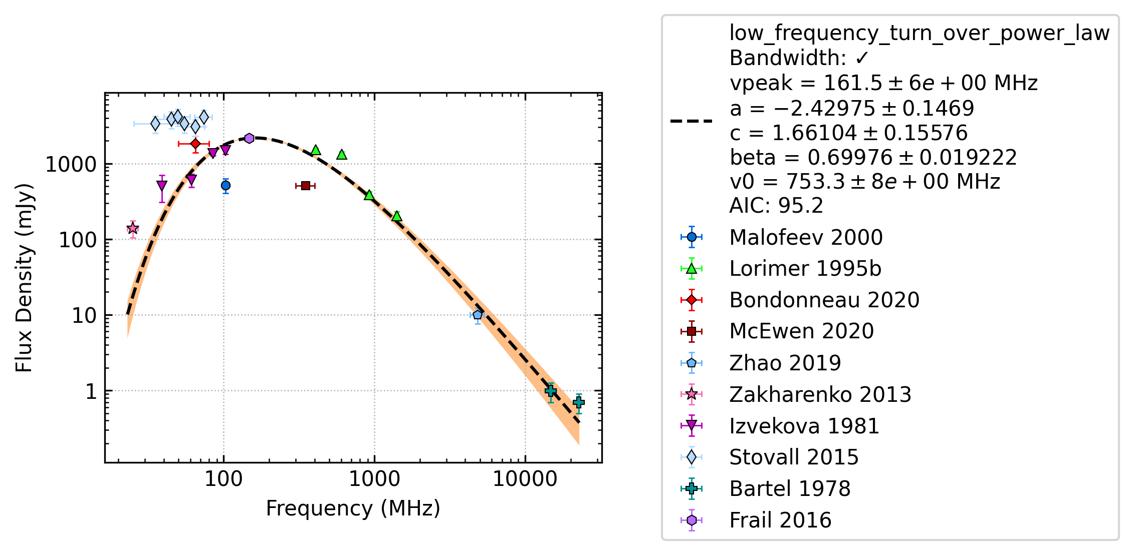
This will produce J0332+5434_low_frequency_turn_over_power_law_fit.png
If you would like to see the result of the best fit you can print them like so
print(f"Best fit model: {best_model_name}")
for p, v, e in zip(iminuit_result.parameters, iminuit_result.values, iminuit_result.errors):
    if p.startswith("v"):
        print(f"{p} = {v/1e6:8.1f} +/- {e/1e6:8.1} MHz")
    else:
        print(f"{p} = {v:.5f} +/- {e:.5}")
which will output
Best fit model: low_frequency_turn_over_power_law
vpeak =    161.5 +/-    6e+00 MHz
a = -2.42975 +/- 0.1469
c = 1.66104 +/- 0.15576
beta = 0.69976 +/- 0.019222
v0 =    753.3 +/-    8e+00 MHz
Adding your data
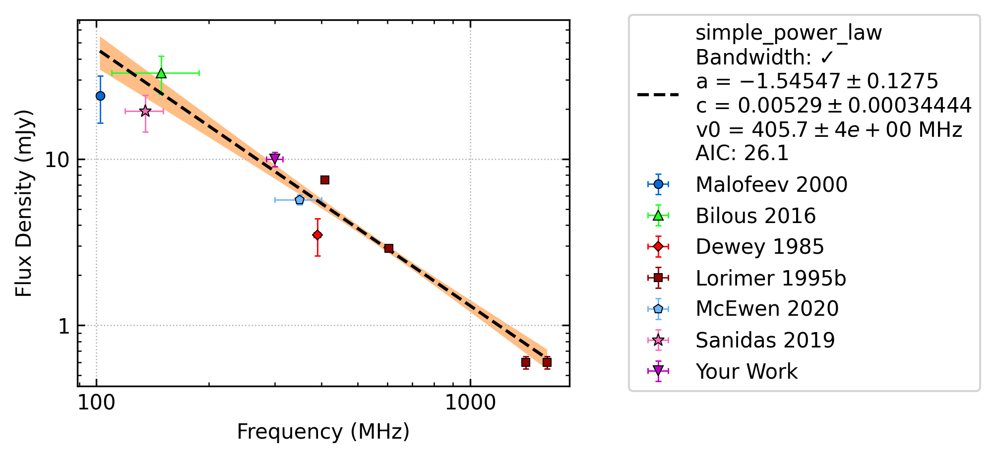
Expanding on the previous example you add your own example like so
from pulsar_spectra.catalogue import collect_catalogue_fluxes
from pulsar_spectra.spectral_fit import find_best_spectral_fit

cat_list = collect_catalogue_fluxes()
pulsar = 'J0040+5716'
freqs, bands, fluxs, flux_errs, refs = cat_list[pulsar]
freqs += [300.]
bands += [30.]
fluxs += [10.]
flux_errs += [2.]
refs += ["Your Work"]
find_best_spectral_fit(pulsar, freqs, bands, fluxs, flux_errs, refs, plot_best=True)
This will also produce J0040+5716_simple_power_law_fit.png with your data included in the fit and plot.
Making a multi pulsar plot
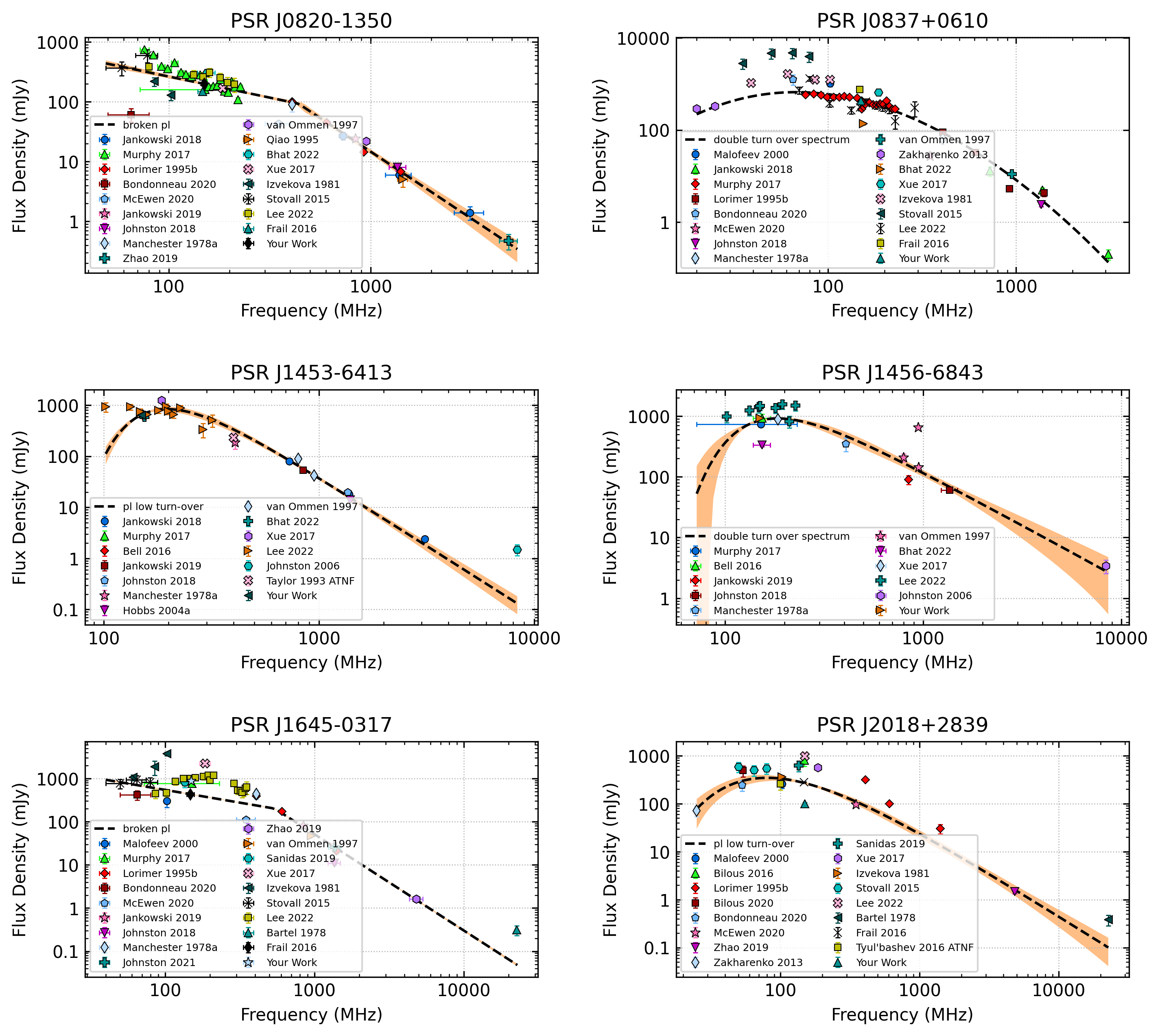
You can create a plot containing multiple pulsars by handing the find_best_spectral_fit a matplotlib axes like so:
import matplotlib.pyplot as plt
from pulsar_spectra.spectral_fit import find_best_spectral_fit
from pulsar_spectra.catalogue import collect_catalogue_fluxes

# Pulsar, flux, flux_err
pulsar_flux = [
    ('J0820-1350', 200, 9,  0),
    ('J0837+0610', 430, 10, 1),
    ('J1453-6413', 630, 20, 2),
    ('J1456-6843', 930, 25, 3),
    ('J1645-0317', 883, 80, 4),
    ('J2018+2839', 100, 10, 5),
]
cols = 2
rows = 3
fig, axs = plt.subplots(nrows=rows, ncols=cols, figsize=(5*cols, 3*rows))

cat_dict = collect_catalogue_fluxes()
for pulsar, flux, flux_err, ax_i in pulsar_flux:
    freqs, bands, fluxs, flux_errs, refs = cat_list[pulsar]
    freqs += [150.]
    bands += [10.]
    fluxs += [flux]
    flux_errs += [flux_err]
    refs += ["Your Work"]

    model, m, fit_info, p_best, p_category = find_best_spectral_fit(pulsar, freqs, bands, fluxs, flux_errs, refs, plot_best=True, alternate_style=True, axis=axs[ax_i//cols, ax_i%cols])
    axs[ax_i//cols, ax_i%cols].set_title('PSR '+pulsar)

plt.tight_layout(pad=2.5)
plt.savefig("multi_pulsar_spectra.png", bbox_inches='tight', dpi=300)
This will produce the following plot.
Estimate flux density
You can use the pulsar’s fit to estimate a pulsar’s flux density at a certain frequency like so:
from pulsar_spectra.spectral_fit import find_best_spectral_fit, estimate_flux_density
from pulsar_spectra.catalogue import collect_catalogue_fluxes

cat_dict = collect_catalogue_fluxes()
pulsar = 'J0820-1350'
freqs, bands, fluxs, flux_errs, refs = cat_list[pulsar]
model, m, _, _, _ = find_best_spectral_fit(pulsar, freqs, bands, fluxs, flux_errs, refs, plot_best=True)
fitted_flux, fitted_flux_err = estimate_flux_density(150., model, m)
print(f"{pulsar} estimated flux: {fitted_flux:.1f} ± {fitted_flux_err:.1f} mJy")
Which will output
J0820-1350 estimated flux: 197.6 ± 11.6 mJy
Calculate the peak frequency for a log parabolic spectrum fit
Log parabolic spectrum is no longer used by default. If you turn it back on, you can use the pulsar’s fit to calculate the peak frequency like so:
from pulsar_spectra.spectral_fit import find_best_spectral_fit
from pulsar_spectra.catalogue import collect_catalogue_fluxes
from pulsar_spectra.analysis import calc_log_parabolic_spectrum_max_freq

cat_dict = collect_catalogue_fluxes()
pulsar = 'J1136+1551'
freqs, bands, fluxs, flux_errs, refs = cat_dict[pulsar]
model_name, m, _, _, _ = find_best_spectral_fit(pulsar, freqs, bands, fluxs, flux_errs, refs)
if model_name == "log_parabolic_spectrum":
    v_peak, u_v_peak = calc_log_parabolic_spectrum_max_freq(
        m.values["a"],
        m.values["b"],
        m.values["v0"],
        m.errors["a"],
        m.errors["b"],
        m.covariance[0][1],
    )
    print(f"v_peak (MHz): {v_peak/1e6:6.2f} +/- {u_v_peak/1e6:6.2f}")
else:
    print("Not a log parabolic spectrum fit")
Which will output
v_peak (MHz): 99.77 +/- 6.51
Estimate emission height from a high-frequency cut-off power-law fit
As demonstrated in Jankowski et al. (2018), we can use the high-frequency cut-off power-law model from Kontorovich & Flanchick (2013) to estimate the location of the centre of the magnetic polar cap, assuming a canonical neutron star (radius of 12+/-2 km; Steiner et al., 2018) and a dipole magnetic field. To perform this calculation, use the in-built function as follows:
from pulsar_spectra.spectral_fit import find_best_spectral_fit
from pulsar_spectra.catalogue import collect_catalogue_fluxes
from pulsar_spectra.models import calc_high_frequency_cutoff_emission_height

cat_dict = collect_catalogue_fluxes()
pulsar = 'J0452-1759'
freqs, bands, fluxs, flux_errs, refs = cat_dict[pulsar]
model_name, m, _, _, _ = find_best_spectral_fit(pulsar, freqs, bands, fluxs, flux_errs, refs)
if model_name == "high_frequency_cut_off_power_law":
    B_pc, u_B_pc, B_surf, B_lc, r_lc, z_e, u_z_e, z_percent, u_z_percent = calc_high_frequency_cutoff_emission_height(
        pulsar,
        m.values[0],
        m.errors[0],
    )
    print(f"B_pc:    ({B_pc/1e11:.2f} +/- {u_B_pc/1e11:.2f})x10^11 G")
    print(f"B_surf:  {B_surf/1e12:.2f}x10^12 G")
    print(f"B_LC:    {B_lc:.2f} G")
    print(f"R_LC:    {r_lc:.0f} km")
    print(f"z_e:     {z_e:.1f} +/- {u_z_e:.1f} km")
    print(f"z/R_LC:  {z_percent:.2f} +/- {u_z_percent:.2f} %")
else:
    print("Not a power-law with high-frequency cut-off fit")
Which will output
B_pc:    (0.22 +/- 0.01)x10^11 G
B_surf:  1.80x10^12 G
B_LC:    101.92 G
R_LC:    26184 km
z_e:     52.0 +/- 8.7 km
z/R_LC:  0.20 +/- 0.03 %