Spectral fit
The pulsar spectral fitting is explained in Swainston et al. 2022 and based on Jankowski et al. 2018. We will summarise how the fitting is done and examples of how to improve your fits.
Fitting algorithm
To account for underestimated uncertainties on outlier points, we modify the regular least-squared quadratic loss function to deviate to linear loss once a certain distance is reached from the model. In this way, outlier data are penalised, and bad data is less likely to skew the model fit. We use the Huber loss function, which is defined as
where \(t\) is a residual and \(k\) is a constant (which we set to 1.345) that defines the point at which outlying points are penalised.
The code will use mingrad function from the iminuit Python package is used to find the minimum of the cost function. This uses a maximum of 10000 calls to converge with the Estimated Distance to Minimum (EDM) criterion. We set the tolerance so that the EDM must be less than \(0.0000002 * errordef\).
In the rare cases that migrad does not find a valid fit, we then try the simplex and scan minimisation methods. Simplex does not use derivatives, making it slower but can perform better in some instances. Scan is a brute-force minimisation that uses a grid of possible solutions based on the limits of the input parameters.
The uncertainties were computed using hesse, an error calculator which computes the covariance matrix for the fitted parameters and determines
the \(1\sigma\) uncertainties as the square root of the diagonal elements.
This is all done within the pulsar_spectra.spectral_fit.iminuit_fit_spectral_model() function.
Models
This fit is done for all functions in the models module that are included in pulsar_spectra.models.model_settings().
If you would like to use a new model, you can add a function to the models’ module and set up the defaults for its
initial fit parameters and limits in pulsar_spectra.models.model_settings().
You can also change the defaults for other models to attempt to improve the fit.
Make sure you reinstall pulsar_spectra to apply any changes you have made to pulsar_spectra.models.model_settings()
Best fit
The best fit model is determined using the Akaike information criterion (AIC), which measures how much information the model retains about the data without overfitting. It was implemented as
where \(\beta_\mathrm{min}\) is the minimised robust cost function, \(K\) is the number of free parameters, and \(N\) is the number of data points in the fit. The last term is the correction for finite sample sizes, which goes to zero as the sample size gets sufficiently large. The model which results in the lowest AIC is the most likely to be the best fitting model.
All of this is done by calling the pulsar_spectra.spectral_fit.find_best_spectral_fit() function like so:
from pulsar_spectra.catalogue import collect_catalogue_fluxes
from pulsar_spectra.spectral_fit import find_best_spectral_fit

cat_dict = collect_catalogue_fluxes()
pulsar = 'J1453-6413'
freqs, fluxs, flux_errs, refs = cat_dict[pulsar]
best_model_name, iminuit_result, fit_info, p_best, p_category = find_best_spectral_fit(pulsar, freqs, fluxs, flux_errs, refs, plot_best=True)
To confirm that the best model has been found, you can visually inspect the fits of all models using the plot_compare option like so
best_model_name, iminuit_result, fit_info, p_best, p_category = find_best_spectral_fit(pulsar, freqs, fluxs, flux_errs, refs, plot_compare=True)
which will produce
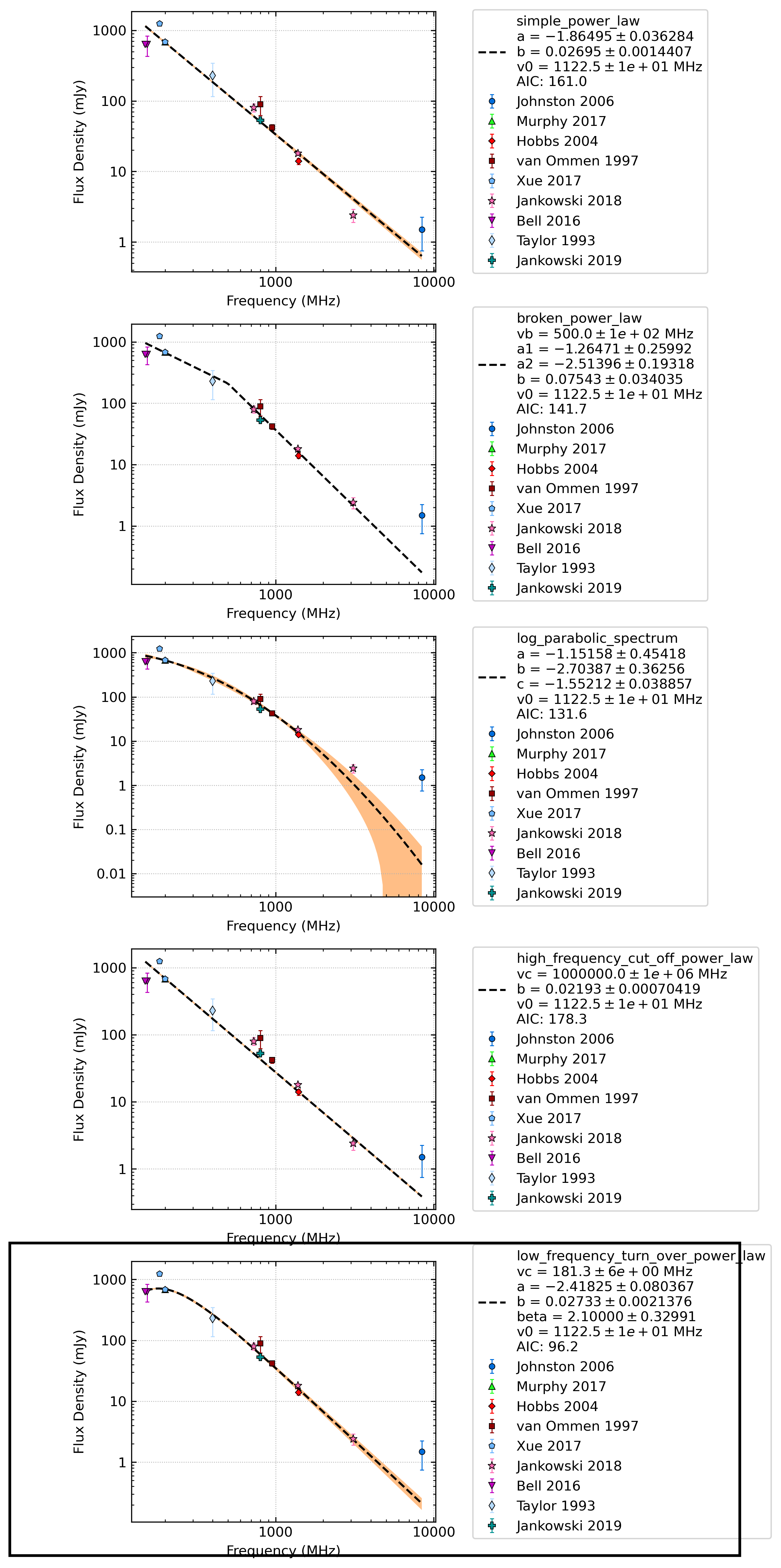
From this plot, it does look like the power-law with a low-frequency turnover is the best model as the code predicted.
If this is not the case and wanted to try and improve the broken power-law fit, for example, you can have more control over the
fit using pulsar_spectra.spectral_fit.iminuit_fit_spectral_model() function like so.
from pulsar_spectra.catalogue import collect_catalogue_fluxes
from pulsar_spectra.spectral_fit import iminuit_fit_spectral_model

cat_list = collect_catalogue_fluxes()
pulsar = 'J1453-6413'
freqs, fluxs, flux_errs, refs = cat_list[pulsar]

# Broken power law function is in the format
# broken_power_law(v, vb, a1, a2, b, v0)

# start params for (v, vb, a1, a2, b)
start_params = (5e8, -1.6, -1.6, 0.1)

# Fit param limits (min, max) or (v, vb, a1, a2, b)
mod_limits = [(None, None), (-10, 10), (-10, 0), (0, None)]
# None means there is no limit

aic, iminuit_result, fit_info = iminuit_fit_spectral_model(
    freqs,
    fluxs,
    flux_errs,
    refs,
    model_name="broken_power_law",
    start_params=start_params,
    mod_limits=mod_limits,
    plot=True,
    save_name="J1453-6413_broken_power_law.png",
)
In this example we are manually handing pulsar_spectra.spectral_fit.iminuit_fit_spectral_model() the default
start_params and mod_limits but you can edit these.